Week 9
Social Statistics and
Machine Learning

SOCI 316

Sakeef M. Karim
Amherst College

SOCIAL RESEARCH

Demystifying Regressions—
March 24^th

Let’s Fit a Linear Probability Model

Caveat Emptor

Using a linear probability model (LPM) to predict a binary outcome can produce predicted probabilities—P(Y=1\mid X)—that fall outside the [0, 1] interval.

Let’s Fit a Linear Probability Model

We’re going to fit one anyway
(cf. von Hippel 2015).

Our Case

Full Page

Our Task

To predict the probability of surviving the sinking of the Titanic as
a function of predictors like age, sex and passenger class.

P(\text{Survival} = 1 \mid X) = \beta_0 + X\beta + \varepsilon

A Simple Bivariate Model

Our Truncated Sample

titanic <- carData::TitanicSurvival |> 
           rownames_to_column(var = "name") |> 
           as_tibble() |> 
           mutate(survived = as.numeric(survived) - 1) 

set.seed(905)

titanic_subset <- titanic |> 
                  slice_sample(n = 3, by = passengerClass) |> 
                  select(name, survived, age)

titanic_subset

# A tibble: 9 × 3
  name                            survived   age
  <chr>                              <dbl> <dbl>
1 Aubart, Mme. Leontine Pauline          1    24
2 Stone, Mrs. George Nelson (Mart        1    62
3 Cardeza, Mr. Thomas Drake Marti        1    36
4 Buss, Miss. Kate                       1    36
5 Smith, Miss. Marion Elsie              1    40
6 Hocking, Mr. Richard George            0    23
7 Cohen, Mr. Gurshon Gus                 1    18
8 Cribb, Mr. John Hatfield               0    44
9 Skoog, Miss. Mabel                     0     9

Our First Model

P(\text{Survival} = 1 \mid X) = \beta_0 + \beta_1\text{age} + \varepsilon

We’re modelling the probability of survival as a function of age.

Our First Model

To fit this model, we need to calculate the slope and intercept parameters—that is, \beta_0 and \beta_1\text{age}, respectively.

Slopes can be derived using the following formula—

b = \frac{\sum{(X - \bar{X})(Y - \bar{Y})}}{\sum{(X - \bar{X})^2}}

Intercepts can be calculated as follows—

\alpha = \bar{Y} - b\bar{X}

Our First Model

Plugging in Our Values

• Step 1: Slope
• Step 2: Intercept

Y	X	X - \bar{X}	Y - \bar{Y}	(X - \bar{X})(Y - \bar{Y})	(X - \bar{X})^2
1	24	-8.44	0.33	-2.81	71.31
1	62	29.56	0.33	9.85	873.53
1	36	3.56	0.33	1.19	12.64
1	36	3.56	0.33	1.19	12.64
1	40	7.56	0.33	2.52	57.09
0	23	-9.44	-0.67	6.33	89.14
1	18	-14.44	0.33	-4.81	208.53
0	44	11.56	-0.67	-7.74	133.64
0	9	-23.44	-0.67	15.67	549.64
		\sum (X - \bar{X}) = 0	\sum (Y - \bar{Y}) = 0	\sum (X - \bar{X})(Y - \bar{Y}) = 21.33	\sum (X - \bar{X})^2 = 2008.92

\beta_1 = \frac{21.33}{2008.92} \approx 0.0106

\beta_0 = 0.667 - (0.0106 \times 32.44) \approx 0.3220

Our first LPM can therefore be summarized as follows—

\hat{P}(\text{Survived} = 1) = 0.3220 + 0.0106 \cdot \text{age} + \varepsilon

Our First Model

Plugging in Our Values

We can use programs like to streamline hand calculations.

library(tidyverse)

titanic_subset |> mutate(# Averages
                         mean_y = mean(survived),
                         mean_x = mean(age),
                         # To establish covariation between x and y
                         # Deviations from average, x
                         x_minus_mean_x = age - mean(age),
                         # Corresponding y value--deviations from average
                         y_minus_mean_y = survived - mean(mean_y),
                         # Tapping co-movement
                         slope_numerator = x_minus_mean_x * y_minus_mean_y,
                         # Squared residuals, positive values are yielded
                         slope_denominator = x_minus_mean_x^2) |> 
                         # Putting it all together
                  mutate(# Summing up the values for the numerator ...
                         slope_numerator = sum(slope_numerator),
                         # And the denominator ...
                         slope_denominator = sum(slope_denominator),
                         # Yielding the slope estimate
                         slope = slope_numerator/slope_denominator,
                         # Which allows us to "solve" for the intercept:
                         intercept = mean_y - slope * mean_x) |> 
                  select(intercept, slope) |> 
                  distinct()

# A tibble: 1 × 2
  intercept  slope
      <dbl>  <dbl>
1     0.322 0.0106

And thankfully, get around doing hand calculations in the first place.

lm(survived ~ age, data = titanic_subset)

Call:
lm(formula = survived ~ age, data = titanic_subset)

Coefficients:
(Intercept)          age  
    0.32201      0.01062  

Let’s Use Our Model—A Case Study

Kate Buss was 36 years old when the Titanic sank.

# A tibble: 1 × 3
  name             survived   age
  <chr>               <dbl> <dbl>
1 Buss, Miss. Kate        1    36

We can compute her probability of survival—using our clearly misspecified model—as follows:

0.32201 + (0.01062 * 36) 

[1] 0.70433

Or we can use functions to generate these predictions for us.

survival_truncated <- lm(survived ~ age, data = titanic_subset) 

titanic_subset |> 
# No measures of uncertainty here
mutate(estimate = predict(survival_truncated)) |> 
slice(4)

# A tibble: 1 × 4
  name             survived   age estimate
  <chr>               <dbl> <dbl>    <dbl>
1 Buss, Miss. Kate        1    36    0.704

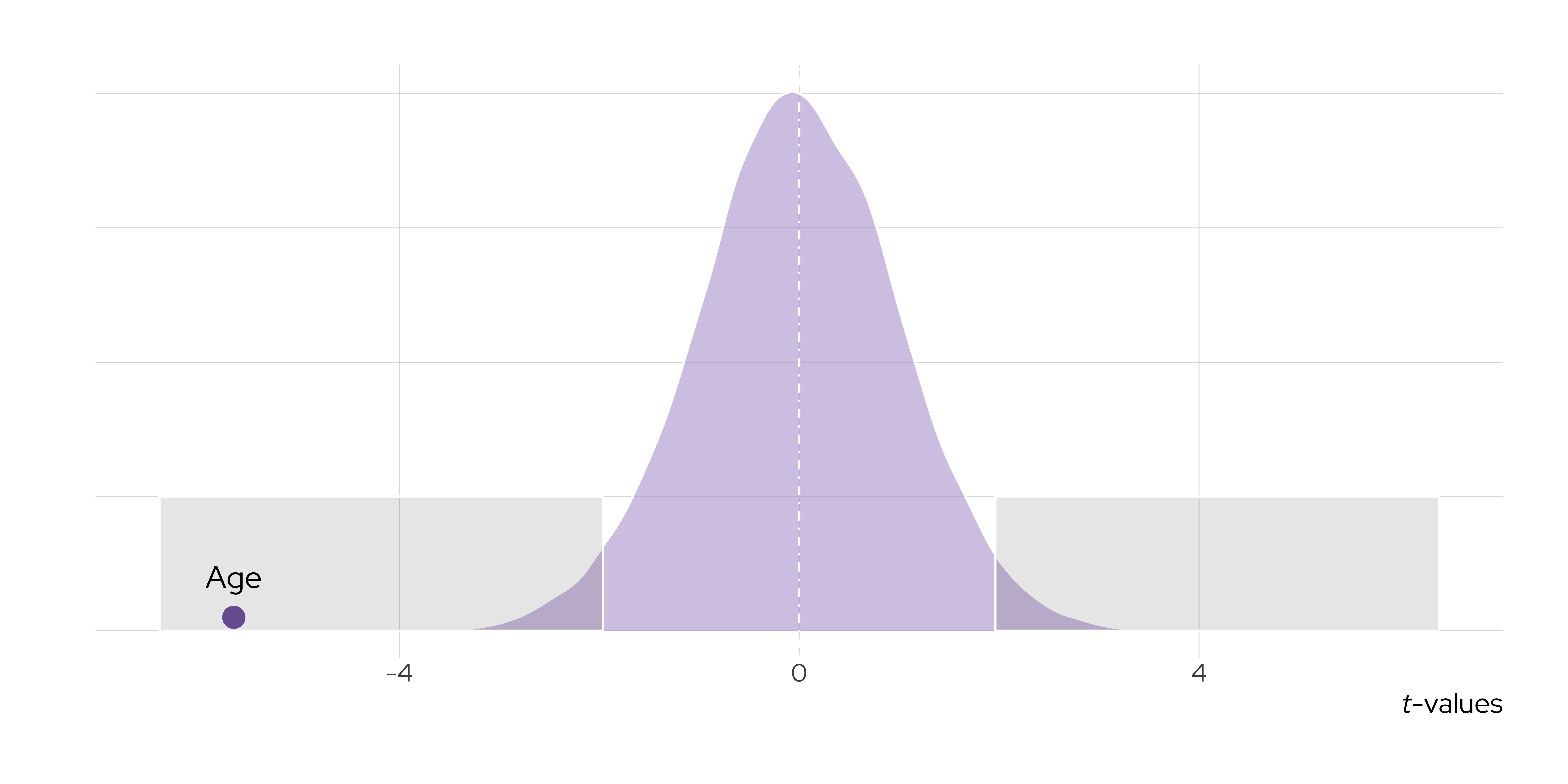
Let’s Use Our Model

Range of Predictions—Truncated Sample

library(marginaleffects)


avg_predictions(survival_truncated, variables = "age") |> 
as_tibble() |> 
ggplot(mapping = aes(x = age, y = estimate)) +
geom_line(colour = "#b7a5d3", linewidth = 1.1) +
geom_ribbon(mapping = aes(ymin = conf.low,
                          ymax = conf.high),
            fill = "lightgrey",
            alpha = 0.3) +
theme_bw()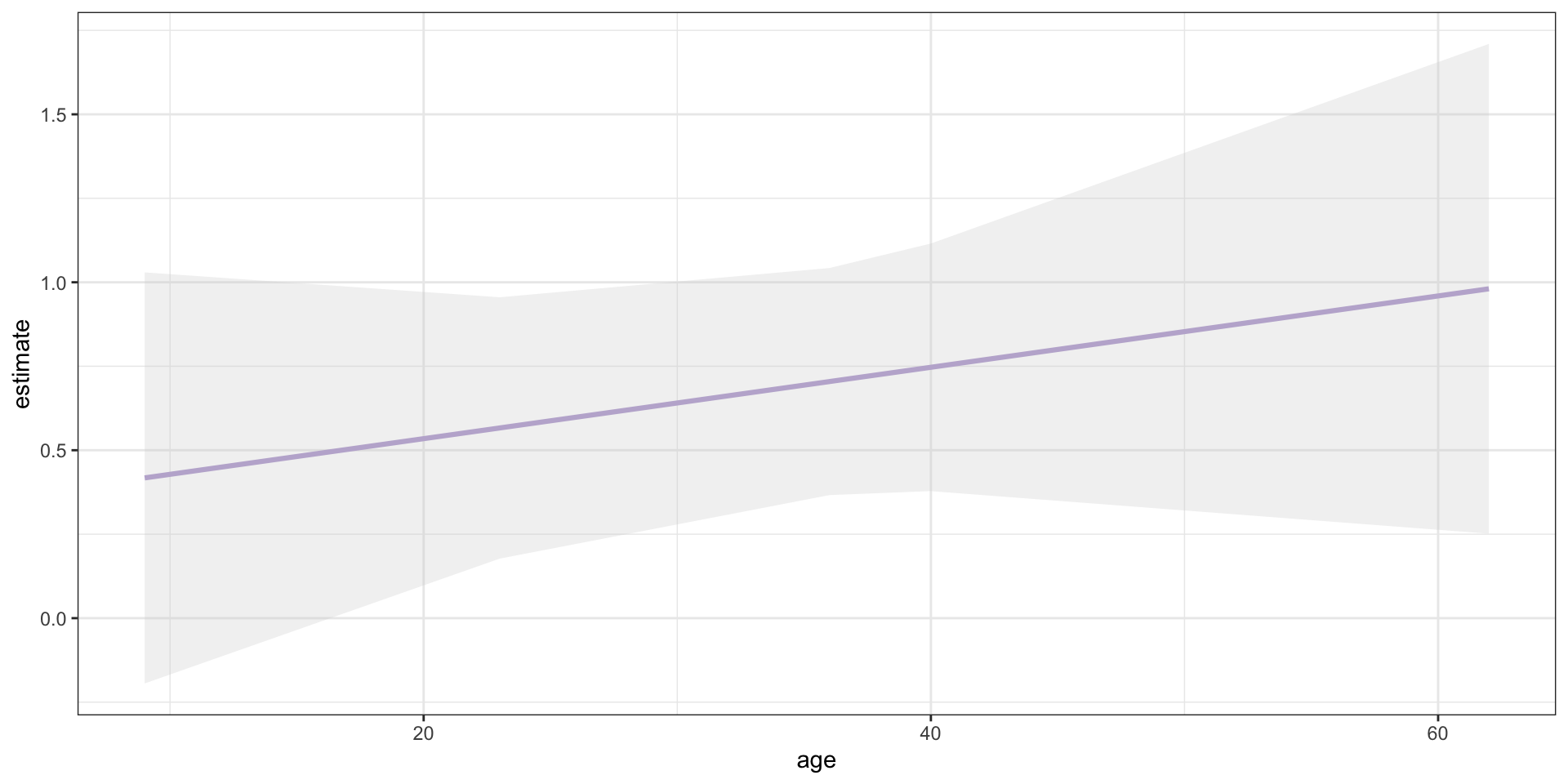

Let’s Use Our Model

Range of Predictions—Full Sample

survival_full <- lm(survived ~ age, data = titanic) 

avg_predictions(survival_full, variables = "age") |> 
as_tibble() |> 
ggplot(mapping = aes(x = age, y = estimate)) +
geom_line(colour = "#b7a5d3", linewidth = 1.1) +
geom_ribbon(mapping = aes(ymin = conf.low,
                          ymax = conf.high),
            fill = "lightgrey",
            alpha = 0.3) +
theme_bw()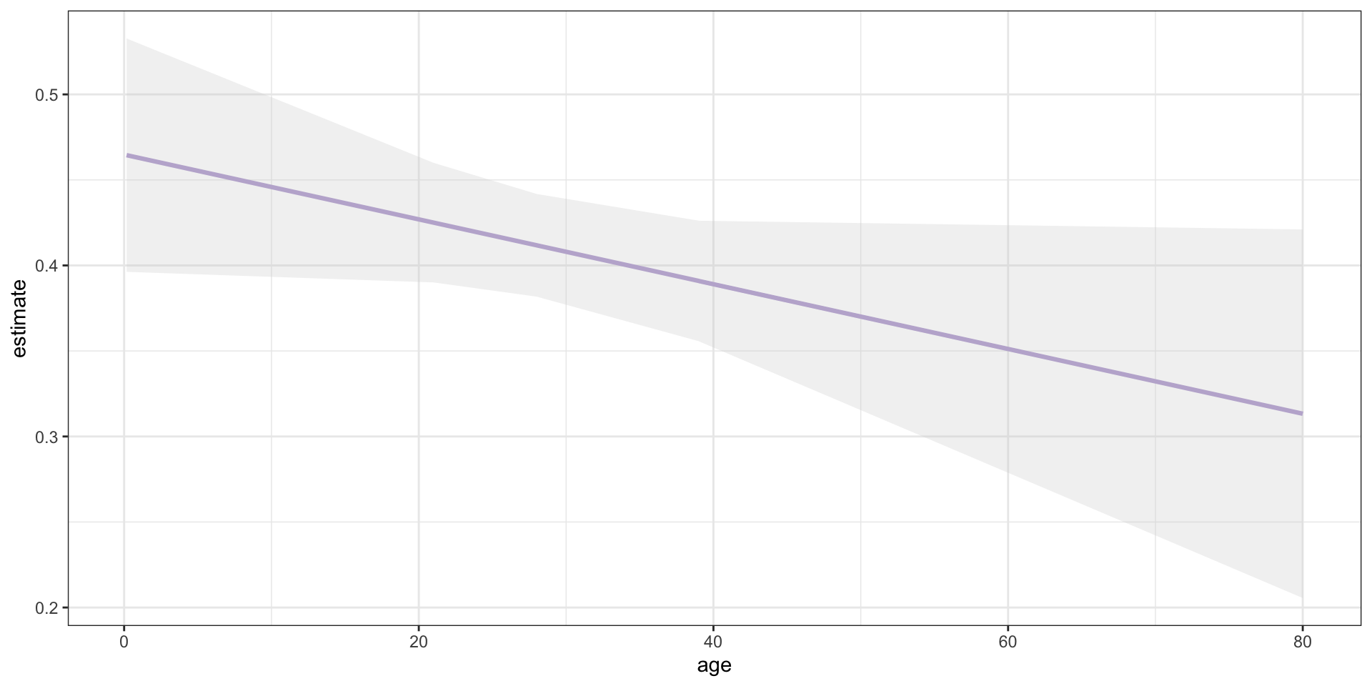

Let’s Use Our Model

Whoops!

Adding More Predictors

Updating the Full Model

update(survival_full, . ~ . + sex + passengerClass) |> 
summary()

Call:
lm(formula = survived ~ age + sex + passengerClass, data = titanic)

Residuals:
     Min       1Q   Median       3Q      Max 
-1.09442 -0.24408 -0.08375  0.23289  0.99397 

Coefficients:
                    Estimate Std. Error t value Pr(>|t|)    
(Intercept)        1.1049549  0.0438210  25.215  < 2e-16 ***
age               -0.0052695  0.0009316  -5.656 2.00e-08 ***
sexmale           -0.4914131  0.0255520 -19.232  < 2e-16 ***
passengerClass2nd -0.2113738  0.0348568  -6.064 1.85e-09 ***
passengerClass3rd -0.3703874  0.0325039 -11.395  < 2e-16 ***
---
Signif. codes:  0 '***' 0.001 '**' 0.01 '*' 0.05 '.' 0.1 ' ' 1

Residual standard error: 0.3913 on 1041 degrees of freedom
  (263 observations deleted due to missingness)
Multiple R-squared:  0.3691,    Adjusted R-squared:  0.3667 
F-statistic: 152.3 on 4 and 1041 DF,  p-value: < 2.2e-16

Updating the Full Model

\begin{align*} \hat{P}(\text{Survived} = 1) = 1.105 - 0.00527 \cdot \text{age} - 0.4914 \cdot \text{sex}_\text{male} \\ - 0.2114 \cdot \text{class}_\text{2nd} - 0.3704 \cdot \text{class}_\text{3rd} + \varepsilon \end{align*}

Call:
lm(formula = survived ~ age + sex + passengerClass, data = titanic)

Coefficients:
      (Intercept)                age            sexmale  passengerClass2nd  
         1.104955          -0.005269          -0.491413          -0.211374  
passengerClass3rd  
        -0.370387  

We’re now modelling the probability of survival as a function of age, sex and passenger class.

Group Exercise I

Making Predictions

Here are three passengers selected at random:

# A tibble: 3 × 5
  name                            survived sex     age passengerClass
  <chr>                              <dbl> <fct> <dbl> <fct>         
1 Veal, Mr. James                        0 male     40 2nd           
2 Petersen, Mr. Marius                   0 male     24 3rd           
3 Johnson, Master. Harold Theodor        1 male      4 3rd           

In groups of 2-3, calculate the probability of survival for each passenger.

Call:
lm(formula = survived ~ age + sex + passengerClass, data = titanic)

Coefficients:
      (Intercept)                age            sexmale  passengerClass2nd  
         1.104955          -0.005269          -0.491413          -0.211374  
passengerClass3rd  
        -0.370387  

The “Solution”

Scroll for the code.

# A tibble: 3 × 2
  name                            estimate
  <chr>                              <dbl>
1 Veal, Mr. James                    0.191
2 Petersen, Mr. Marius               0.117
3 Johnson, Master. Harold Theodor    0.222

x <- c(24, 4)

c(1.104955 - 0.491413 - 0.211374 - (40 * 0.005269),
  map_dbl(x, ~  1.104955 - 0.491413 - 0.370387 - (. * 0.005269)))

[1] 0.191408 0.116699 0.222079

A Note About Uncertainty

Meaning in the Stars

stargazer::stargazer(survival_full, type = "text")

===============================================
                        Dependent variable:    
                    ---------------------------
                             survived          
-----------------------------------------------
age                          -0.005***         
                              (0.001)          
                                               
sexmale                      -0.491***         
                              (0.026)          
                                               
passengerClass2nd            -0.211***         
                              (0.035)          
                                               
passengerClass3rd            -0.370***         
                              (0.033)          
                                               
Constant                     1.105***          
                              (0.044)          
                                               
-----------------------------------------------
Observations                   1,046           
R2                             0.369           
Adjusted R2                    0.367           
Residual Std. Error      0.391 (df = 1041)     
F Statistic          152.257*** (df = 4; 1041) 
===============================================
Note:               *p<0.1; **p<0.05; ***p<0.01

Standard Errors

SE(\hat{\beta}) = \sqrt{\frac{\hat{\sigma}^2}{\sum_{i = 1}^n (x_i- \bar{x})^2}}

Parameter estimates based on our full model.

# A tibble: 1 × 5
  term  estimate std.error statistic      p.value
  <chr>    <dbl>     <dbl>     <dbl>        <dbl>
1 age   -0.00527  0.000932     -5.66 0.0000000155

Test Statistic Values

Hypothesis Testing

In Standard OLS Settings

t = \frac{\hat{\beta} - \color{856cb0}{\beta_{H_\theta}}}{SE(\hat{\beta})}

Hypothesis Testing

In Standard OLS Settings

t = \frac{\hat{\beta} - \color{856cb0}{\beta_{H_0}}}{SE(\hat{\beta})}

survival_full |> 
broom::tidy() |> 
filter(term == "age") |> 
mutate(manual_statistic = (estimate - 0)/std.error,
       .after = statistic)

# A tibble: 1 × 6
  term  estimate std.error statistic manual_statistic      p.value
  <chr>    <dbl>     <dbl>     <dbl>            <dbl>        <dbl>
1 age   -0.00527  0.000932     -5.66            -5.66 0.0000000200

Statistical Significance

According to Your Textbook

A result is statistically significant at the 5% level when the corresponding parameter is distinguishable from zero using 5% as the rejection threshold. Conversely, a result is not statistically significant at the 5% level when the corresponding parameter is not distinguishable from zero using 5% as the rejection threshold.

(Llaudet and Imai 2023, 215, EMPHASIS ADDED)

Memo II

Five Survey Items

Your next assignment is due this Friday at 8:00 PM. As a refresher—you are required to submit a short response memo proposing five potential survey questions.

For each question, you must include a \approx 100-word rationale explaining how the proposed item addresses a significant sociological question.

Please use the rest of today’s session to work on the memo!

A Gentle Introduction to Machine Learning—
March 27^th

Informal Presentations

Full Page

An Invitation

A Talk by Dr. Julian Go

Title

Policing Empires

Abstract

Click to Expand or Close

In the US and Britain, police bear the weapons and mindsets of armies, manifesting a “militarization” of policing. This lecture by Professor Julian Go offers a historical sociology of police militarization, revealing how, when and why it has occurred. It reveals what we call “police militarization” has been happening since the very founding of modern policing in the nineteenth century.

Date and Time

  March 31^st — 5:00 PM to 7:00 PM

Location

  CHI Think Tank (101) at the Lyceum

What is Machine Learning?

Some Concrete Definitions

Grimmer and colleagues (2021, 396, EMPHASIS ADDED)

A class of flexible algorithmic and statistical techniques for prediction and dimension reduction.

Molina and Garip (2019, 28, EMPHASIS ADDED)

A way to learn from data and estimate complex functions that discover representations of some input (X), or link the input to an output (Y) in order to make predictions on new data.

Supervised Machine Learning (SML)

High-Level Overview

• Once deployed, SML algorithms learn the complex patterns linking X—a set of features (or independent variables)—to a target variable (or outcome), Y.

  • The goal of SML is to optimize predictions—i.e., to find functions or algorithms that offer substantial predictive power when confronted with new or unseen data.

  • Examples of SML algorithms include logistic regressions, random forests, ridge regressions, support vector machines and neural networks.

• A quick note on terminology

  • If a target variable is quantitative, we are dealing with a regression problem.

  • If a target variable is qualitative, we are dealing with a classification problem.

Supervised Machine Learning (SML) cont.

An Illustration

• (1) Feed Input Data
• (2) Develop Algorithm
• (3) Predictions on New Data

# A tibble: 80,000 × 6
   fruit      shape       weight_g colour texture origin    
   <chr>      <chr>          <dbl> <chr>  <chr>   <chr>     
 1 apple      spherical        150 red    crispy  china     
 2 banana     curved           120 yellow creamy  ecuador   
 3 orange     spherical        148 orange juicy   egypt     
 4 watermelon spherical       4500 green  juicy   spain     
 5 strawberry conical           13 red    juicy   mexico    
 6 grape      spherical          5 green  juicy   chile     
 7 mango      ellipsoidal      240 yellow juicy   india     
 8 pineapple  conical         2100 yellow juicy   costa rica
 9 apple      spherical        140 green  crispy  usa       
10 banana     curved           110 yellow creamy  ecuador   
# ℹ 79,990 more rows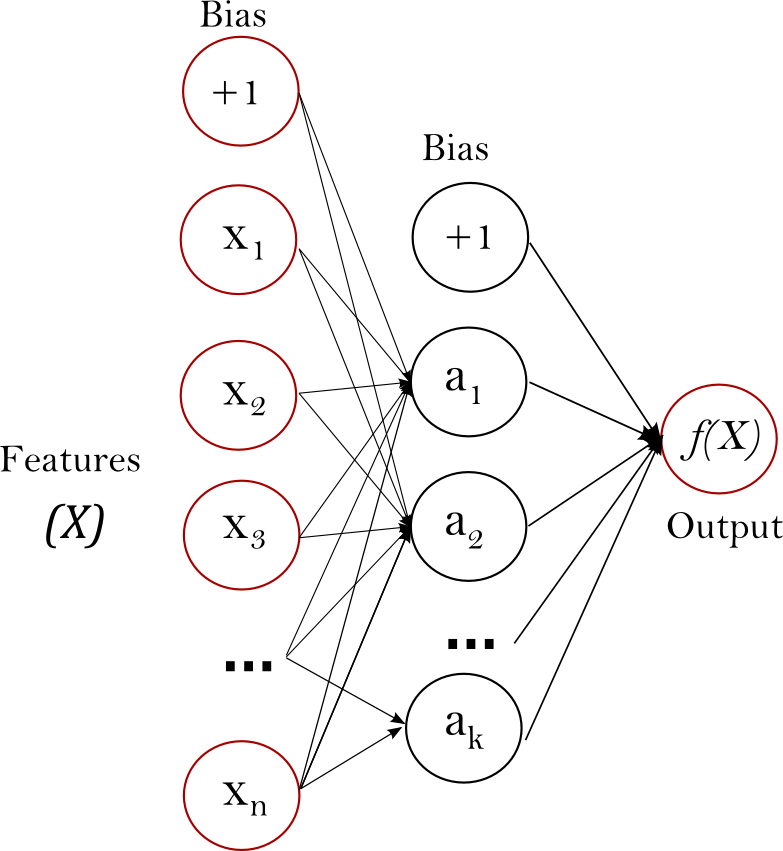

via scikit-learn

# A tibble: 1 × 6
  fruit shape   weight_g colour texture origin
  <chr> <chr>      <int> <chr>  <chr>   <chr> 
1 <NA>  conical        6 red    juicy   china 

# A tibble: 8 × 2
  fruit      probability
  <chr>            <dbl>
1 apple             0.03
2 banana            0   
3 orange            0.05
4 watermelon        0   
5 strawberry        0.71
6 grape             0.21
7 mango             0   
8 pineapple         0   

# A tibble: 1 × 1
  prediction
  <chr>     
1 strawberry

Strawberry icons created by BZZRINCANTATION - Flaticon

Unsupervised Machine Learning (UML)

High-Level Overview

• UML techniques search for a representation of the inputs (or features) that is more useful than X itself (Molina and Garip 2019).

  • Put another way, UML algorithms search for hidden structure or latent patterns in high dimensional space.

• In UML, there is no observed outcome variable Y—or target—to supervise the estimation process. Instead, we only have a vector of inputs to work with.

• The goal in UML is to develop a lower-dimensional representation of complex data by inductively learning from the interrelationships among inputs.

  • This can be achieved by reducing a vector of features to a smaller set of scales (e.g., via principal component analysis) or partitioning the sample into a small number of unobserved groups (e.g., via k-means clustering).

Unsupervised Machine Learning (UML) cont.

An Illustration

V-Party Name	Label	Underlying Question
v2paanteli	Anti-Elitism	How important is anti-elite rhetoric for this party?
v2papeople	People-Centrism	Do leaders of this party glorify the ordinary people and identify themselves as part of them?
v2paculsup	Cultural Chauvinism	To what extent does the party leadership promote the cultural superiority of a specific social group or the nation as a whole?
v2paminor	Minority Rights	According to the leadership of this party, how often should the will of the majority be implemented even if doing so would violate the rights of minorities?
v2paplur	Political Pluralism	Prior to this election, to what extent was the leadership of this political party clearly committed to free and fair elections with multiple parties, freedom of speech, media, assembly and association?
v2paopresp	Demonization of Opponents	Prior to this election, have leaders of this party used severe personal attacks or tactics of demonization against their opponents?
v2paviol	Rejection of Political Violence	To what extent does the leadership of this party explicitly discourage the use of violence against domestic political opponents?

Unsupervised Machine Learning (UML) cont.

An Illustration

Karim and Lukk’s The Radicalization of Mainstream Parties in the 21^st Century

Machine Learning vs Classical Parametric Statistics

The Two Cultures

• As Grimmer and colleagues (2021) note, “machine learning is as much a culture defined by a distinct set of values and tools as it is a set of algorithms.”

• This point has, of course, been made elsewhere.

  • Leo Breiman (2001) famously used the imagery of warring cultures to describe two major traditions—(i) the generative modelling culture and (ii) the predictive modelling culture—that have achieved hegemony within the world of statistical modelling.

  • The terms generative and predictive (as opposed to data and algorithmic) come from David Donoho’s (2017) 50 Years of Data Science.

The Two Cultures cont.

Quantity of Interest	Primary Goals	Key Strengths	Key Limitations
Generative (i.e., Classical Statistics)
	Inferring relationships between X and Y	Interpretability; emphasis on uncertainty around estimates; explanatory power	Bounded by statistical assumptions, inattention to variance across samples
Predictive (i.e., Machine Learning)
	Generating accurate predictions of Y	Predictive power; potential to simplify high dimensional data; relatively unconstrained by statistical assumptions	Inattention to explanatory processes, opaque links between X and Y

Note: To be sure, the putative strengths and weaknesses of these modelling “cultures” have been hotly debated.

The Affordances of Machine Learning

• Advances in machine learning can provide empirical leverage to social scientists and sharpen social theory in one fell swoop.

• Lundberg, Brand and Jeon (2022), for instance, argue that adopting a machine learning framework can help social scientists:

  • Amplify human coding
  • Summarize complex data structures
  • Relax statistical assumptions
  • Target researcher attention

• While ML is often associated with induction, van Loon (2022) argues that SML algorithms can help us deductively resolve predictability hypotheses as well.

  • What plays a larger role in shaping human behaviour—nature or nurture?

Key Terms and Concepts in the SML Setting

Bias-Variance Tradeoff

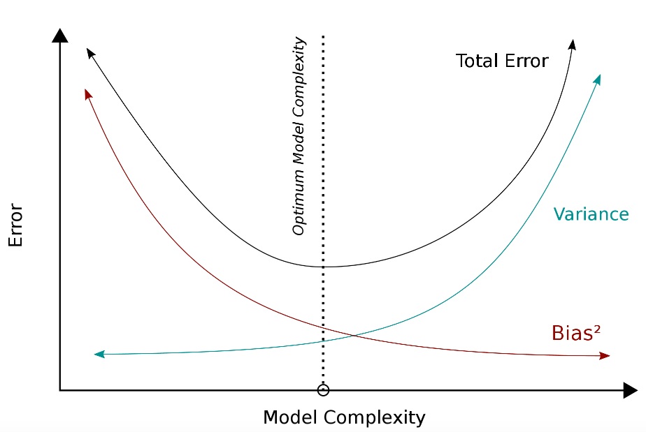
Image can be retrieved here.

• Bias emerges when we build SML algorithms that fail to sufficiently map the patterns—or pick up the empirical signal–linking X and Y. Think: underfitting.

• Variance arises when our algorithms not only pick up the signal linking X and Y, but some of the noise in our data as well. Think: overfitting.

• When adopting an SML framework, researchers try to strike the optimal balance between bias and variance.

Training, Validation and Testing

• In an SML setting, we want to reduce our algorithm’s generalization or test error—i.e., “the prediction error of a model on new data” (Molina and Garip 2019).

• To arrive at an estimate of our model’s performance, we can (randomly) partition our global sample of observations into disjoint sets or subsamples.

• Training
• Validation
• Testing

• We can use a training set to fit our algorithm—to find weights (or coefficients), recursively split the feature space to grow decision trees and so on.

• Training data should constitute the largest of our three disjoint sets.

• We can use a validation set to find the right estimator out of a series of candidate algorithms—or select the best-fitting parameterization of a single algorithm.

• Often, using both training and validation sets can be costly: data sparsity can give rise to bias.

• Thus, when limited to smaller samples, analysts often combine training and validation—say, by recycling training data for model tuning and selection.

• We can use a testing set to generate a measure of our model’s predictive accuracy (e.g., the F1 score for classification problems)—or to derive our generalization error.

• This subsample is used only once (to report the performance metric); put another way, it cannot be used to train, tune or select our algorithm.

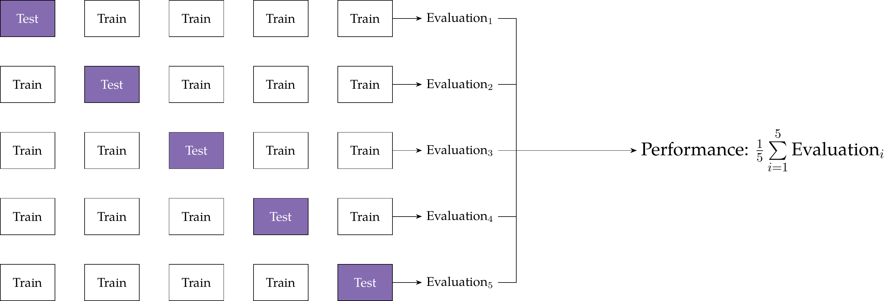
k-Fold Cross-Validation

• High-Level Overview
• An Illustration

• Unlike conventional approaches to sample partition, k or v-fold cross-validation allows us to learn from all our data.

• k-fold cross-validation proceeds as follows:

  • We randomly divide our overall sample into k subsets or folds.
  • We train our algorithm on k - 1 folds, holding just one group out for model assessment.
  • We repeat this process k times—every fold is held out once and used to fit the model k - 1 times.
  • We then pool or average the evaluation metrics (e.g., predictive accuracy) for all the held-out runs.

• Stratified k-fold cross-validation ensures that the distribution of class labels (or for numeric targets, the mean) is relatively constant across folds.

Stylized example of five-fold cross-validation

Hyperparameter Optimization

• In SML settings, we automatically learn the parameters (e.g., coefficients) of our algorithms during estimation.

• Hyperparameters, on the other hand, are chosen by the analyst, guide the entire learning or estimation process, and can powerfully shape our algorithm’s predictive performance.

  • Examples of hyperparameters include the k in nearest neighbours algorithms, the \alpha penalty term in ridge regressions, or the number of hidden layers in a neural network.

• How can analysts settle on the right hyperparameter value(s) for their algorithm?

  • Test different values via trial and error.
  • Use automated procedures like GridSearchCV from scikit-learn.

k-Nearest Neighbours

Brief Overview of KNN

• k-nearest neighbours (KNNs) are simple, non-parametric algorithms that predict values of Y based on the distance between rows (or observations’ inputs).

• The estimation of KNNs proceeds as follows:

  • The analyst defines the distance metric (e.g., Euclidean, Manhattan) they will use to determine how similar any two observations are based on their vector of features.
  • The analyst defines a value for the hyperparameter k—that is, the number of nearest neighbours to find in the training subsample.
    
  • When fed a new data point, KNNs find the k nearest neighbours in the training data, and:
    • Assign the new observation to the class that most of its k nearest neighbours belong to (for classification problems.)
      
    • Generate a prediction of Y by taking the average of the target variable for the new observation’s k nearest neighbours (for regression problems.)
      

KNN in Python

# Importing pandas to wrangle the data, modules from scikit-learn to fit KNN classifier,
# and numpy to iterate over potential values of k (for a grid search):

import pandas as pd 

from sklearn.model_selection import train_test_split, cross_val_score, StratifiedKFold, GridSearchCV

from sklearn.preprocessing import StandardScaler

from sklearn.neighbors import KNeighborsClassifier

import numpy as np

# Load input data frame:

gapminder = pd.read_excel("https://github.com/sakeefkarim/intro.python.24/raw/main/data/gapminder.xlsx")

# Homing-in on observations in the latest year (2007)

gapminder = gapminder.query("year == 2007").reset_index(drop=True).drop(columns='year')

# Generating dummy indicator indexing whether a country is in Asia:

gapminder['asia'] = pd.get_dummies(gapminder['continent'])['Asia']

# Removing target variable and categorical indicators from feature vector:

X = gapminder.drop(columns = ['asia', 'continent', 'country'])

# Isolating target variable:

y = gapminder['asia']

# Perform train-test split:

X_train, X_test, y_train, y_test = train_test_split(X, y, stratify = y, test_size = 0.15, random_state = 905)

# Standardizing feature data

sc = StandardScaler()

# Applied to training data

X_train = sc.fit_transform(X_train)

# Applied to test data

X_test = sc.transform(X_test)

# Initializing KNN classifier with k = 5, fitting model:

knn = KNeighborsClassifier(n_neighbors = 5).fit(X_train, y_train)

# Stratified k-fold cross-validation:

skfold = StratifiedKFold(n_splits = 5, shuffle = True, random_state = 905)

# Cross-validation score:

knn_5_cv = cross_val_score(knn, X_train, y_train, cv = skfold).mean()

# Measure of predictive performance:

knn_5_test = knn.score(X_test, y_test)

print(f"Cross-Validation Score: {knn_5_cv:.3f},\nTest Set Score: {knn_5_test:.3f}")

Cross-Validation Score: 0.792,
Test Set Score: 0.818

# Creating a grid of potential hyperparameter values (odd numbers from 1 to 13):

k_grid = {'n_neighbors': np.arange(start = 1, stop = 14, step = 2) }

# Setting up a grid search to home-in on best value of k:

grid = GridSearchCV(KNeighborsClassifier(), param_grid = k_grid, cv = skfold)

grid_fit = grid.fit(X_train, y_train)

print(f"Best Mean Cross-Validation Score: {grid.best_score_:.3f},\nBest Parameters (Value of k): {grid.best_params_},\nTest Set Score: {grid.score(X_test, y_test):.3f}")

Best Mean Cross-Validation Score: 0.817,
Best Parameters (Value of k): {'n_neighbors': 3},
Test Set Score: 0.773

Note: Keep clicking or the space bar on your to advance through this slide.

Memo II

Five Survey Items

Please use the rest of today’s session to
work on your second response memo!

Enjoy the Weekend

References

Note: Scroll to access the entire bibliography

Breiman, Leo. 2001. “Statistical Modeling: The Two Cultures (with Comments and a Rejoinder by the Author).” Statistical Science 16 (3). https://doi.org/10.1214/ss/1009213726.

Donoho, David. 2017. “50 Years of Data Science.” Journal of Computational and Graphical Statistics 26 (4): 745–66. https://doi.org/10.1080/10618600.2017.1384734.

Grimmer, Justin, Margaret E. Roberts, and Brandon M. Stewart. 2021. “Machine Learning for Social Science: An Agnostic Approach.” Annual Review of Political Science 24 (1): 395–419. https://doi.org/10.1146/annurev-polisci-053119-015921.

Llaudet, Elena, and Kōsuke Imai. 2023. Data Analysis for Social Science: A Friendly and Practical Introduction. Princeton, NJ: Princeton University press.

Lundberg, Ian, Jennie E. Brand, and Nanum Jeon. 2022. “Researcher Reasoning Meets Computational Capacity: Machine Learning for Social Science.” Social Science Research 108 (November): 102807. https://doi.org/10.1016/j.ssresearch.2022.102807.

Molina, Mario, and Filiz Garip. 2019. “Machine Learning for Sociology.” Annual Review of Sociology 45 (Volume 45, 2019): 27–45. https://doi.org/10.1146/annurev-soc-073117-041106.

van Loon, Austin. 2022. “Machine Learning and Deductive Social Science: An Introduction to Predictability Hypotheses.” SocArXiv. https://doi.org/10.31235/osf.io/s7uer.

von Hippel, Paul. 2015. “Linear Vs. Logistic Probability Models: Which Is Better, and When?” Statistical Horizons. https://statisticalhorizons.com/linear-vs-logistic/.